Volatility is arguably the single most important (and most misunderstood) option concept. Volatility at its most basic level is used to describe the distribution of rates of return. In an option context, it is the distribution of rates of return of the underlying security - not of the option itself. Why is volatility so important? Because volatility is synonymous with the value of the option.
If you could forecast the future distribution of returns, you would be able to estimate the current value of every option. If you could forecast implied volatility (IV - the market’s estimate of volatility) in the future, you would be able to estimate the future value of volatility indices and the future value of every option. If your estimates of the future return distribution and future implied volatilities diverged materially from the market’s estimates, you could design option and volatility index futures strategies to exploit those targeted pricing anomalies and earn excess risk-adjusted returns.
I have studied, researched, and modeled volatility for my entire 30+ year career as an investment professional: institutional investment manager, Professor of Practice, and proprietary trader. Forecasting future volatility is an extremely complex challenge.
I have devoted the last year to designing a comprehensive option volatility forecasting platform called AI Volatility Edge - which is an integrated collection of AI models based on the latest machine-learning (ML) algorithms. The AI Volatility Edge platform is available on a subscription basis for professional and non-professional traders.
If you have previously registered on the Trader Edge site, please use the email link you receive after ordering to register again. Please use a different email address during registration to ensure your AIVE PayPal payment profile is linked to your new registration.
Please note that a NEW version of the AIVE platform is now available and IS compatible with 64-bit versions of Excel!
The original AIVE platform is available for use with 32-bit versions of Excel (even if installed on a 64-bit version of Microsoft Windows).
Non-Professional: AI Volatility Edge E-Subscription: $69 / mo.
PROFESSIONAL: AI Volatility Edge E-Subscription: $690 / mo.
AI Models
I have extensive experience with Artificial Intelligence (AI) models, dating back to the late-1990s. During that time, I developed and licensed a suite of neural network models (including a volatility model) used by professional investment managers, including hedge funds, international banks, and mutual fund companies.
AI models are extremely powerful – perhaps too powerful. It is almost too easy to provide a machine learning algorithm with a wide range of input data, push a button, and have it spit out a trained model with seemingly accurate estimates. AI models excel at modeling non-linear, correlated, complex data relationships. Without expert oversight and design, they will overfit the training data – essentially memorizing the data, rather than generalizing the underlying data relationships. The resulting models will fail in practice, which is very costly in financial modeling.
To make matters worse, unlike an expert system, it is not possible to precisely trace the software logic of an AI model and understand exactly how and why it will respond to all future events. There have already been several catastrophic and deadly failures of self-driving technology and there will be more.
It is simply not possible to “debug” AI models, but they are too valuable to ignore. The only practical solution is to integrate knowledge of markets, algorithmic trading, and machine learning to manage and constrain the AI model design, training, and application.
The first step in the design process is to drastically limit the number and choice of input variables to ensure that each of the explanatory variables has a material cause-and-effect relationship with the forecasted variable. The AI Volatility Edge models all use fewer than 10 input variables, one of which is the score from the Trader Edge Option Income Strategy Universal Filter (OISUF) algorithm.
To further reduce the number of input variables, all models use the same proprietary variables, rather than cherry-picking the explanatory variables for each model to artificially improve the fit. In addition, the training set was constrained to a small fraction of the entire data set; a much larger data set was withheld for testing and validation, encouraging the models to generalize. The unique design of the model is based on fundamental cause-and-effect relationships, which allowed me to build a single aggregate volatility model for the RUT, NDX, and the SPX, rather than separate models for each index. This effectively tripled the number of data observations, further encouraging the models to generalize and capture the underlying cause-and-effect relationships in the data. During the training process, the number of training/optimization iterations was severely constrained to reduce overfitting. All of the above techniques were employed to ensure the most robust possible set of volatility models.
One of the pioneering insights I had back in the 1990s was to aggregate the results from several AI models together to arrive at a consensus estimate, rather than rely on the results from a single model. I employed the same technique when designing the AI Volatility Edge platform. Each volatility forecast represents the weighted-average of the results from three different models, each with a different structure and/or learning algorithm (but the same training set and input variables). Aggregating the individual model forecasts reduces outliers and typically has better out-of-sample error statistics than any of the three individual models.
AI Volatility Edge
Before we get into a detailed description of the AI Volatility Edge platform, I want to address one important point. You may be concerned about the complexity of the model. The design of the AI models is complex, but the user interface in Excel is easy to use and understand - with push-button macros and simple tables and graphs. Most important, the interpretation of the volatility forecasts is straightforward. If volatility forecasts were higher than anticipated, volatility would be expected to rise (suggesting long volatility strategies) and vice versa. Several detailed examples with actual market data and specific strategies will be presented later to demonstrate how the AIVE forecasts could be interpreted and applied in practice.
The AI Volatility Edge platform forecasts four different types of future volatility (explained in detail below): annualized Realized Volatility (RV), Volatility index prices (VX), Realized Terminal Volatility (RTV), and Realized Extreme Volatility (REV), each for a specific number of trade days into the future: 0, 5, 10, 15, 21, 31, 42, 63, 84, 105, 126, 189, 252, and 504. The RV, VX, and RTV forecasts are derived from 80 different AI models (three for each time period and type of volatility). The Realized Extreme Volatility forecast is estimated using a regression model based on the AI model forecasts.
Realized Volatility (RV) is the annualized volatility derived from the daily returns of the underlying equity index over a specified number of trading days in the future. It can be compared directly to the implied volatility of at-the-money (ATM) options.
If realized volatility forecasts were higher than the at-the-money (ATM) volatilities of the equity index options, then ATM options would potentially be undervalued. In this environment, positive Gamma strategies would be desirable to capitalize on higher than expected realized volatility. If the realized volatility forecasts were lower than the volatilities of ATM equity index options, then ATM options would potentially be overvalued, which would suggest negative Gamma/Positive Theta strategies.
The AI Volatility Edge platform also forecasts the volatility index prices (VX) a specified number of trading days into the future. These values are directly comparable to the current prices of volatility index futures contracts on the corresponding expiration dates.
If volatility index forecasts were higher than volatility index futures prices, then volatility index futures would potentially be undervalued. Since volatility index prices are derived from actual options, this is equivalent to saying that implied volatilities would be expected to rise more than anticipated, which would advocate positive Vega strategies. If the volatility index forecasts were lower than volatility index futures prices, then volatility index futures would potentially be overvalued. In this environment, future implied volatilities would be lower than expected, which would suggest negative Vega strategies. Obviously, volatility index futures or options on volatility index futures could also be used to capitalize on these prospective VX anomalies as well.
The AI Volatility Edge platform also forecasts Realized Terminal Volatility (RTV), which represents the expected continuously compounded percentage price change of the underlying equity index from the analysis date to the end of the specified period in the future. These return forecasts are not annualized and are not directional. In other words, a 21-trade day RTV forecast of 4% would imply an expected price change of plus or minus 4% (continuously compounded) from now until the close, 21 trading days in the future.
The Realized Extreme Volatility (REV) is an estimate of the maximum percentage price change of the underlying equity index at any time during the specified period in the future. As was the case with the Realized Terminal Volatility, the Realized Extreme Volatility forecasts are not annualized and are not directional. If the Realized Terminal Volatility forecast was plus or minus 4% for the next 21 days, the Realized Extreme Volatility forecast might be plus or minus 5.6% (continuously compounded). The RTV and REV are extremely useful when designing option strategies, especially selecting strike prices.
Running the AI Volatility Edge Models
There are only four steps in the AI Volatility Edge Analysis: 1) import the input data, 2) generate the model forecasts, 3) enter the current IV and VX futures data, and 4) analyze the results. I have provided links to two demonstration videos of the AI Volatility Edge Analysis below and I strongly encourage you to review the first video before reading the remainder of this document. Seeing a dynamic demonstration of the spreadsheet, while listening to an explanation would help provide a foundation for the written description that follows.
AI Volatility Edge Video Demo #1: Overview
AI Volatility Edge Video Demo #2: User Interface (I/O)
The AI Volatility Edge models use proprietary variables derived from current and historical equity price and volatility index data to generate their forecasts. The AIVE spreadsheets have two import options. The first option imports data from price and IV data files that were previously downloaded for free from Yahoo and the CBOE respectively. The second option imports data from price and IV data files that are downloaded daily from Commodity Systems Inc. (CSI), the data-vendor that I use for all of my trading and research. There is also an option to enter the intra-day price and volatility index data, to generate real-time volatility forecasts. All of these import options are fully automated with push-button macros in the spreadsheets.
The next step is to choose an analysis date (current or historical) and calculate all of the volatility forecasts – again using a simple push-button macro. The user could quickly compare the volatility forecasts to a specific market implied volatility or volatility index futures price of interest, but it is much more valuable to evaluate the entire term structure of volatilities.
This requires current at-the-money (ATM) implied volatilities for equity options and current volatility index futures data (if available) for the specific equity volatility index. This real-time data is available through all broker platforms and through option analytics vendors such as OptionVue. If your broker has an Excel DDE API, it would be possible to enter links in the AI Volatility Edge spreadsheets to update these values in real-time.
Finally, the Analysis worksheet compares the market IV and futures data with the AI Volatility Edge forecasts in graphical and tabular format to help identify prospective pricing anomalies.
Overpriced Volatility Example
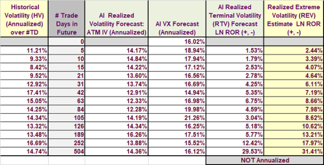
The easiest way to understand the AI Volatility Edge platform is through specific examples (using static screen shots below and in the dynamic video demos). All of the tables and graphs shown below are available in the AI Volatility Edge spreadsheets. The first example uses closing prices from October 1, 2019. Figure 1 below lists all forecasts from the AI Volatility Edge models on 10/1/2019. The actual annualized historical volatilities are provided for the specified number of trading days in the past (0, 5, 10, … 504) and the Realized Volatility (RV), VX Forecast, Realized Terminal Volatility (RTV), and Realized Extreme Volatility (REV) forecasts are provided for the specified number of trading days in the future (0, 5, 10, … 504). This list of trading days is fixed. The general forecast data below will be used to generate specific forecasts that correspond to the expiration dates of actual equity options and volatility index futures contracts on a separate worksheet.
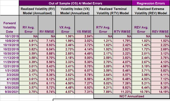
In order to apply the AI Volatility Edge forecasts in practice, we need to know the magnitude of the out-of-sample errors for each model, for each period. This will allow us to consistently evaluate the magnitude of the divergences between market and forecast data for all models, across all time periods. The error table is shown below in Figure 2.
The AI Volatility Edge Platform also includes the “Estimate TSV” worksheet (not shown). This worksheet will be included with Brian Johnson's upcoming book, but also shares commonalities with the AI Volatility Edge Analysis. This optional worksheet uses Solver to calculate the implied forward term structure of volatilities from the IV of ATM equity index options and from volatility index futures prices (if available). The resulting implied term structure of volatilities is then used to calculate a relative value snapshot of each ATM option and volatility index futures contract at a specific point in time. Note, this analysis only uses current ATM IVs and futures prices to calculate an instantaneous relative value analysis. It does not use AI and does not make forecasts. It uses the mathematical relationships embedded in the term structure of volatilities, which will be explored in detail in Brian Johnson's upcoming book.
This worksheet may be used independently or in conjunction with the AI Volatility Edge (AIVE) forecasts. If used in conjunction with the AI Volatility Edge forecasts, the analysis date and associated data must be exactly the same as the date and data used in the AIVE forecasts. Data entered here can then be imported directly into the Analysis Worksheet for an AI relative value analysis, or IV and futures market data can be entered directly in the Analysis worksheet.
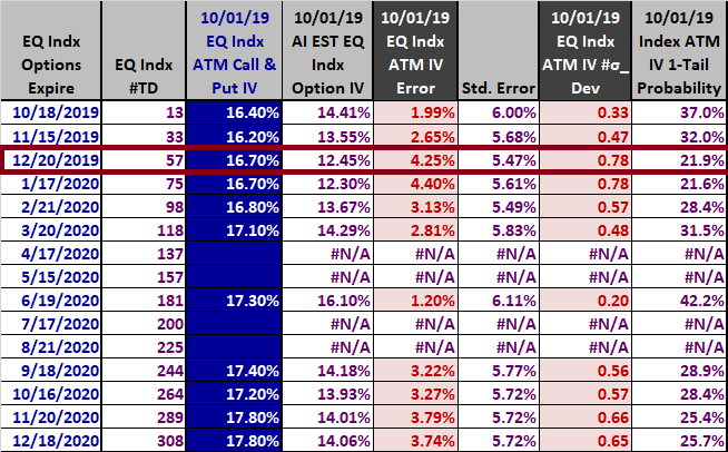
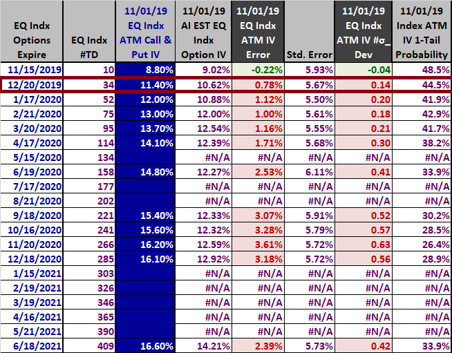
Figure 3 below compares the 10/1/2019 AI Realized Volatility forecasts to the implied volatilities for actual S&P 500 equity index options with a range of expiration dates. Using the highlighted row as an example, the ATM S&P 500 option expires on 12/20/2019, 57 trading days in the future. The annualized implied volatility of that option was 16.70% and the annualized Realized Volatility (RV) forecast was only 12.45%. The resulting option was overpriced by 4.25%. Given a standard error of 5.47%, this error equates to a z-score of + 0.78. In other words, the actual implied volatility exceeded the forecast Realized Volatility by 0.78 standard errors. Calculating z-scores for every instrument allows us to compare the relative value across instruments. Finally, a z-score of 0.78 translates to a one-tailed probability (assuming a normal distribution) of 21.9%. This represents the significance of the observation, specifically the probability of a +0.78 z-score occurring by chance.
Before we begin to evaluate the model results, the first question we always have to ask is whether there is anything unique about the current environment or any known material events that will be occurring in the future that could compromise the forecasts of models derived exclusively from current and historical price and IV data. In this case, I specifically chose a date that was not influenced by upcoming Presidential elections, etc. When those types of near-term events are present, an additional layer of qualitative analysis and judgment is required.
What observations can we make so far? First, the actual implied volatilities exceeded the Realized Volatility forecasts for every ATM option. The entire term structure of ATM implied volatilities was overpriced. Second, the 12/20/2019 expiration was the most overvalued with a z-score of + 0.78. Actually, it was tied with the ATM option expiring on 1/17/2020. This brings up an important point. Regardless of the standard error, near-term forecasts are more reliable than long-term forecasts. It is extremely difficult for any model to generate accurate, reliable volatility forecasts one or two years into the future. Long-term forecasts are provided, and they are derived from quantifiable relationships in the data, but caution is warranted.
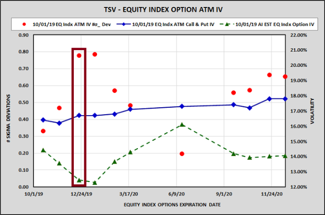
Figure 4 below is a graph of the tabular data presented in Figure 3 above. The dashed-green line represents the volatility forecasts for the series of ATM S&P options, while the solid-blue line represents the actual ATM implied volatilities for the same options. Both of these series use the RHS y-axis. The red dots (LHS y-axis) depict the z-scores or the differences between the actual IVs and the Realized Volatility forecasts, expressed as the number of standard deviations. As is evident in the chart, the z-scores are all positive, indicating the ATM implied volatilities were all overpriced.
This example uses the S&P 500 index, so we also have reliable data for the futures contracts on the corresponding 30-day volatility index – the VIX. Figure 5 below compares the 10/1/2019 AI Volatility Index (VX) forecasts to the VIX futures prices over a range of expiration dates. Using the highlighted row as an example, the VIX futures contract expires on 11/20/2019, 36 trading days in the future. The VIX futures price was 19.18% and the annualized VIX forecast was only 15.90%. The resulting VIX futures contract was overpriced by 3.28%. Given a standard error of 5.14%, this error equates to a z-score of + 0.64. In other words, the actual November 2019 VIX futures price exceeded the 2019 VIX forecast by 0.64 standard errors. Calculating z-scores for every instrument allows us to compare the relative value across instruments. Finally, a z-score of 0.64 translates to a one-tailed probability (assuming a normal distribution) of 26.1%. This represents the significance of the observation, specifically the probability of a +0.64 z-score occurring by chance.
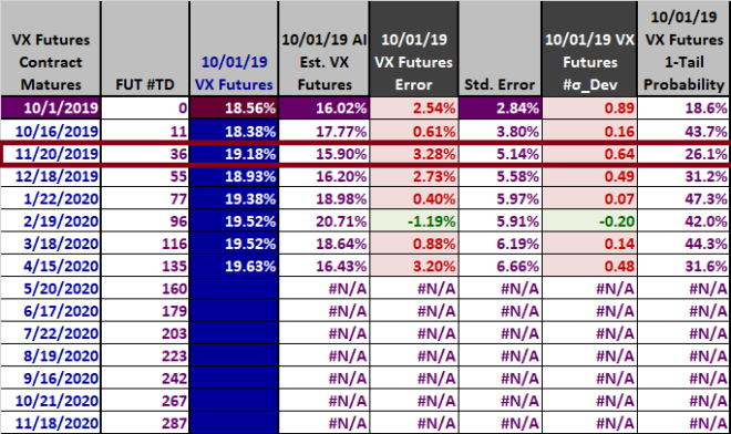
Our observations regarding the VIX futures contracts are similar to the ATM IV analysis. The VIX futures contract prices exceeded the AI VIX futures forecasts for six out of seven futures contracts. The current VIX index value (top row – zero days into the future) also exceeded its forecast. The entire term structure of VIX futures contracts was overpriced. The VIX futures contract expiring on 11/20/2019 was the most overpriced with a z-score of + 0.64. Actually, the current VIX index was more overvalued (higher z-score), but the VIX index itself is not directly tradable.
It is interesting to note that the most overvalued ATM option and most overvalued futures contract are related. The VIX futures contract expiring on 11/20/2019 corresponds to S&P 500 Index options expiring in December - 30 days after the 11/20/2019 expiration date. As you will recall, the 12/20/2019 ATM S&P 500 options were the most overvalued as well. This is particularly encouraging, especially since the models for different volatilities and different dates are entirely unique. They are completely separate models – and they are all generating consistent results. The distinct volatility forecasts for different dates and for the three equity indices should always be compared and contrasted to look for inconsistencies, discrepancies, and outliers before applying the models in practice. For brevity, I will not present the NDX and RUT models here.
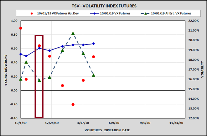
Figure 6 below is a graph of the tabular data presented in Figure 5 above. The dashed-green line represents the VIX forecasts for a series of VIX futures expiration dates, while the solid-blue line represents the VIX futures prices for the same contracts. Both of these series use the RHS y-axis. The red dots (LHS y-axis) depict the z-scores or the differences between the actual VIX futures prices and the VIX forecasts, expressed as the number of standard deviations. As is evident in the chart, the z-scores were all positive (with one minor exception), indicating the VIX futures contracts were overpriced across the entire term structure of volatilities.
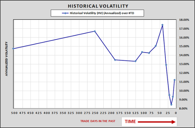
Before we explore specific trades to exploit these prospective pricing anomalies, let’s briefly review the Historical Volatilities as of 10/1/2019. The historical volatilities for the past five to 504 trade days are illustrated graphically in Figure 7. The values are all annualized, so they are directly comparable. As you can see from the graph, historical volatilities peaked over the past 42 trading days (2 months), then declined sharply before picking up slightly in the last five trading days. Recent volatility had been much lower than the volatilities reflected in ATM options and VIX futures.
Overpriced Volatility Trade Entry
The above analysis strongly suggests that the level of volatility priced into ATM equity options and volatility index (VIX) futures on 10/01/2019 was too high – relative to historical relationships between price, implied volatility, and future volatility. This suggests we should attempt to construct trades that have negative Gamma (and therefore positive Theta), which would benefit from a lower than expected level of Realized Volatility, and negative Vega, which would benefit from a prospective decline in implied volatility.
This is the desired environment for employing Option Income Strategies. In my recent book Option Income Trade Filters, I introduced the Option Income Strategy Universal Filter (OISUF) algorithm, which produces a standardized OISUF score.
Scores below zero indicate less favorable OIS environments and scores above zero signify favorable OIS environments. Furthermore, higher OISUF scores imply more advantageous OIS environments across the entire spectrum of prospective OIS values and vice versa. On 10/01/2019, the OISUF score was + 54.06. I intentionally selected a date when the AI Volatility Edge forecast was consistent with an attractive OISUF score. This is not required, but filtering trades based on multiple models is highly effective. Please see the OISUF product page if you would like additional information.
We have identified S&P 500 options expiring on 12/20/2019 and the VIX futures contract expiring on 11/20/2019 as particularly overvalued, so our proposed strategies will focus on these expiration dates in our example strategies.
Let’s begin with an options trade, a simple broken-wing butterfly (BWF), constructed with a put spread and a call spread. The OptionVue Greeks and graphical analysis as of 10/01/2019 are shown in Figures 8 and 9 below, respectively.
I have been a subscriber to OptionVue for many years, but OptionVue is not included with the AIVE subscription. It is a separate product. However, OptionVue does offer a discount for annual OptionVue subscriptions on the TraderEdge.Net site. Please see the RHS side bar for a link to OptionVue.
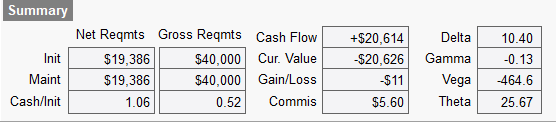
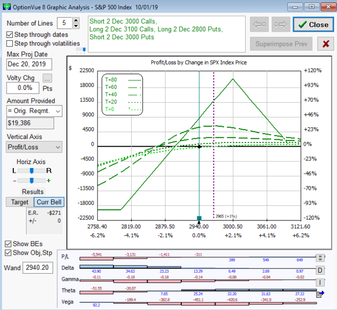
The BWF trade required $19,386 of capital (Reg-T margin) and had the desired negative gamma (-0.13), negative Vega (-464.6) and positive Theta (+25.67), which was consistent with the volatility pricing anomalies implied by the AI Volatility Edge Analysis. You will also note the Delta was also slightly positive (+10.4). That was intentional. Volatility and equity prices are strongly negatively correlated. Given that we are forecasting a decline in volatility, that implies the bias will be toward higher equity prices. This is why I constructed a slightly bullish broken-wing butterfly trade, to be consistent with our volatility forecast. However, keep in mind that the volatility models are not directional; they forecast volatility, not price direction. It is up to the individual trader to determine how or when to leverage the historical relationship between price and volatility.
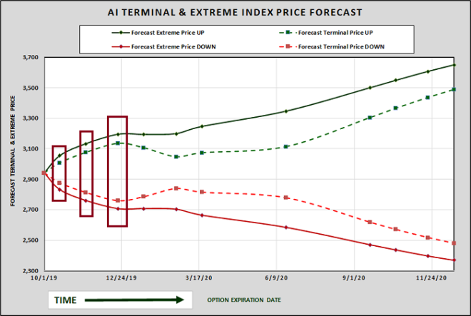
I used the Realized Terminal and Extreme Volatility price chart (Figure 10) below to estimate the potential magnitude of the price changes when selecting the strikes and designing the BWF strategy. The BWF is one of many flavors of Option Income Strategies, which are typically exited well before expiration – to avoid increasing risk due to increases in negative Gamma as the expiration date approaches. As a result, when reviewing the terminal and extreme volatility forecasts, we should focus on the near-term potential holding period, not the expiration date of the options in the strategy.
Overpriced Volatility Trade Exit
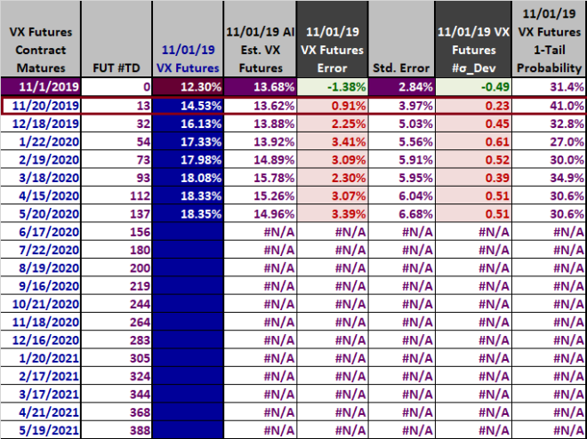
It is not possible to provide a daily analysis of the BWF trade during the holding period, but I will provide a complete analysis on the prospective exit date for the trade: 11/01/2019. Figure 11 below compares the 11/1/2019 AI Realized Volatility forecasts to the implied volatilities for actual S&P 500 equity index options with a range of expiration dates. I have highlighted the same 12/20/2019 options expiration date that we used to construct the BWF trade. As you can see, the ATM IV declined significantly. While it was still slightly overvalued relative to the new volatility forecasts on 11/01/2019, the new z-score had dropped to near zero, which removed most of the edge from our trade.
Similarly, the degree of overvaluation had also declined to near zero for the 11/20/2019 VIX futures contract (Figure 12), which further reinforced the justification for exiting the trade. The term structure of volatilities was still overpriced in general, but not materially for the option expiration dates of interest for our strategy.
You will recall that we used the attractive OISUF score of +54.06 as additional support for entering the BWF trade on 10/1/2019. As of the proposed exit date of 11/1/2019, the OISUF score had dropped to negative 5.24, which would be considered an unattractive OIS environment. The 11/1/2019 AI Volatility Edge forecasts and the OISUF score no longer supported an edge for the BWF trade.
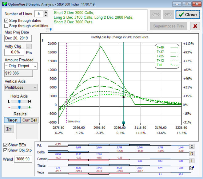
If we look at OptionVue’s graphical analysis (Figure 13) and Greeks (Figure 14) for the BWF trade on 11/01/2019, we also see that we were at the top-end of the sweet-spot of the payoff distribution (which is undesirable) and Delta has turned negative (-14.61), which was inconsistent with the persistent overpriced volatility environment.
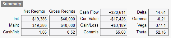
Option trading is inherently a zero-sum game. We should only risk our capital when we have a demonstrated edge. There are definitely anomalies that can be exploited, but when our edge is gone, we should exit the trade. In this case, the trade would have generated a $3,189 profit over the one-month holding period, representing a return on required capital of 16.45%.
Alternative Overpriced Volatility Trades
I will not go into the same level of detail, but I wanted to provide two alternative trades that would have been consistent with the overpriced volatility environment. Note, the interpretation of the Greeks is very different due to the VIX as the underlying index (instead of the S&P 500 index), which I will not explore here. Both alternative trades assume the same entry and exit dates of 10/1/2019 and 11/01/2019, respectively. The first alternative trade was a bear put spread using November 2020 VIX put options (anticipating a decline in the VIX). The OptionVue graphical analysis for the VIX bear put spread on the exit date of 11/1/2019 is shown in Figure 15 and the Greeks summary on the exit date is shown in Figure 16.
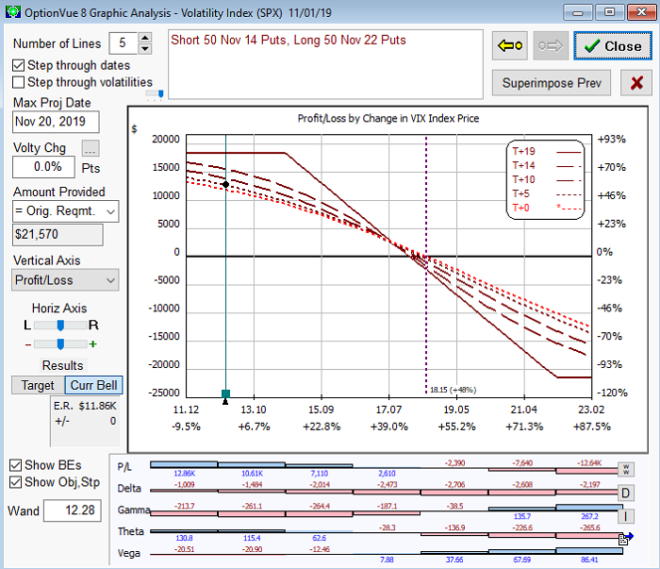
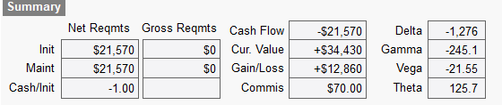
As you can see from the above exhibits, the VIX bear put spread would have earned a profit of $12,860 on a capital requirement of $21,570, which would have resulted in a return on required capital of 59.62% over the one-month holding period.
The second alternative trade was a long November 2020 VIX 14 put option (anticipating a decline in the VIX). The OptionVue Greeks summary for the long VIX put option on the exit date of 11/1/2019 is shown in Figure 17.
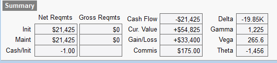
As you can see from the above exhibits, the long VIX put option would have earned a profit of $33,400 on a capital requirement of $21,425, which would have resulted in a return on required capital of 155.89% over the one-month holding period. However, the outright purchase of the VIX put option would have been a much riskier trade, particularly due to the negative Theta of the long VIX put option. However, using VIX futures and VIX options is a very efficient way to implement strategies designed to exploit volatility pricing anomalies, but only for the experienced trader.
One critical comment about short volatility trades; they should ALWAYS be covered. In other words, they should have a maximum possible loss and that maximum loss should be consistent with your account size and degree of risk-aversion. If necessary, hedges should be employed to further reduce the maximum loss if appropriate.
Underpriced Volatility Environment
The next (underpriced volatility) example uses closing prices from November 7, 2018. Figure 18 below lists all forecasts from the AI Volatility Edge models on 11/7/2018. The actual annualized historical volatilities are provided for the specified number of trading days in the past (0, 5, 10, … 504) and the Realized Volatility (RV), VX Forecast, Realized Terminal Volatility (RTV), and Realized Extreme Volatility (REV) forecasts are provided for the specified number of trading days in the future (0, 5, 10, … 504). This list of trading days is fixed. The general forecast data below will be used to generate specific forecasts that correspond to the expiration dates of actual equity options and volatility index futures contracts on a separate worksheet.
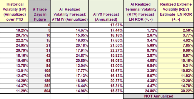
Figure 19 below compares the 11/7/2018 AI Realized Volatility forecasts to the implied volatilities for actual S&P 500 equity index options with a range of expiration dates. Using the highlighted row as an example, the ATM S&P 500 option expires on 01/18/2019, 49 trading days in the future. The annualized implied volatility of that option was 14.50% and the annualized Realized Volatility (RV) forecast was 23.21%. The resulting option was underpriced by 8.71%. Given a standard error of 5.52%, this error equated to a z-score of negative 1.58. In other words, the Realized Volatility forecast exceeded the actual implied volatility by 1.58 standard errors. The corresponding one-tailed probability was only 5.7%.
As was the case in the first example, I specifically chose a date that was not influenced by upcoming Presidential elections, etc. When those types of near-term events are present, an additional layer of qualitative analysis and judgment is always required.
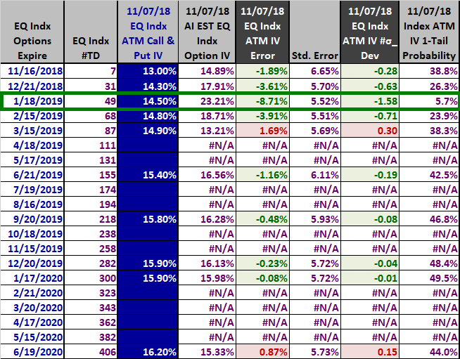
What observations can we make about the term structure of ATM implied volatilities? First, the actual implied volatilities were generally lower than the Realized Volatility forecasts, but there were two exceptions. Second, the 01/18/2019 expiration was the most undervalued with a z-score of negative 1.58, primarily due to a large expected spike in realized volatility. The front three months of the term structure of ATM implied volatilities were the most underpriced.
Figure 20 below is a graph of the tabular data presented in Figure 19 above. The dashed-green line represents the volatility forecasts for the series of ATM S&P options, while the solid-blue line represents the actual ATM implied volatilities for the same options. Both of these series use the RHS y-axis. The red dots (LHS y-axis) depict the z-scores or the differences between the actual IVs and the Realized Volatility forecasts, expressed as the number of standard deviations. As is evident in the chart, the z-scores were primarily negative, indicating many of the ATM implied volatilities were underpriced – particularly the front end of the curve.
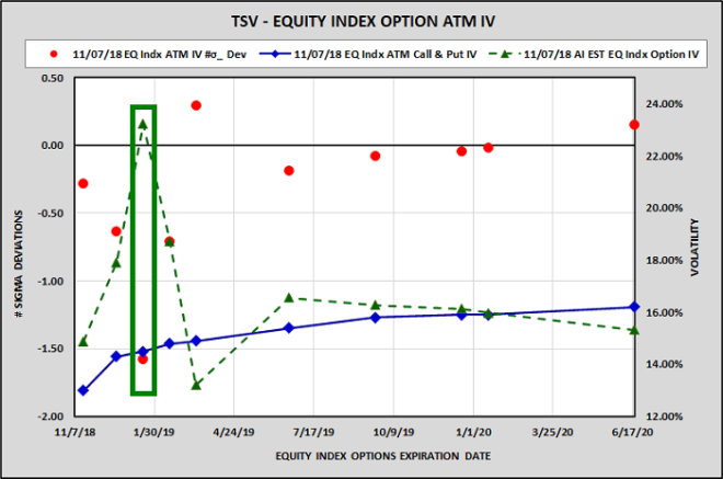
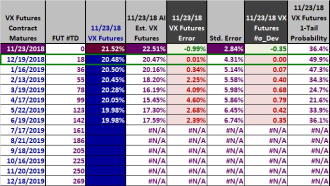
Figure 21 below compares the 11/07/2018 AI Volatility Index (VX) forecasts to the VIX futures prices over a range of expiration dates. Using the highlighted row as an example, the VIX futures contract expires on 12/19/2018, 29 trading days in the future. The VIX futures price was 17.27% and the annualized VIX forecast was 22.13%. The resulting VIX futures contract was underpriced by 4.86%. Given a standard error of 4.90%, this error equates to a z-score of negative 0.99. In other words, the December 2018 VIX forecast exceeded the actual December 2018 VIX futures price by 0.99 standard errors. A z-score of negative 0.99 translates to a one-tailed probability (assuming a normal distribution) of 16.1%.
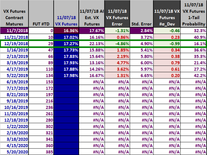
Unlike the ATM IV analysis, the undervaluation of the December 2018 contract appeared to be more of an anomaly, although the VIX index itself was also undervalued. It is interesting to note that the most undervalued ATM option and most undervalued futures contract were related. The VIX futures contract expiring on 12/19/2018 corresponds to S&P 500 Index options expiring in January of 2019 - 30 days after the 12/19/2018 expiration date. As you will recall, the 01/18/2019 ATM S&P 500 options were the most undervalued as well. This same phenomenon occurred in the undervalued option example. This is encouraging because the models for different volatilities and different dates are entirely independent. They are completely separate models – and they are generating consistent results.
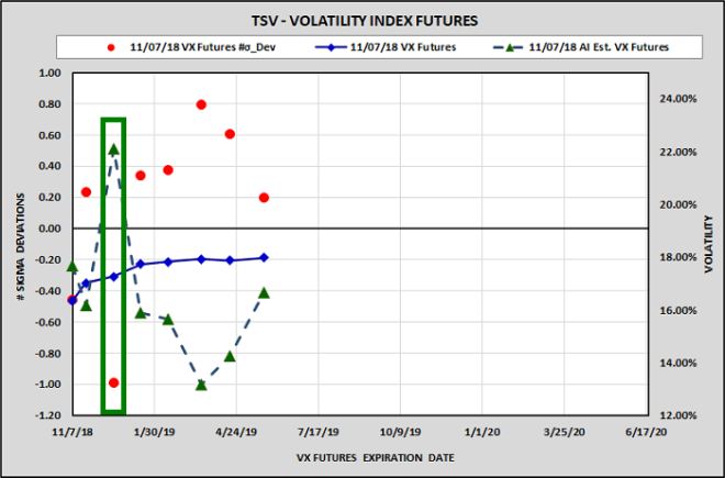
Figure 22 below is a graph of the tabular data presented in Figure 21 above. The dashed-green line represents the VIX forecasts for a series of VIX futures expiration dates, while the solid-blue line represents the VIX futures prices for the same contracts. Both of these series use the RHS y-axis. The red dots (LHS y-axis) depict the z-scores or the differences between the actual VIX futures prices and the VIX forecasts, expressed as the number of standard deviations. As is evident in the chart, many of the z-scores were slightly positive (overvalued), except for the VIX index itself and the December 2019 VIX futures contract, which was significantly negative (underpriced).
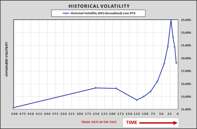
Before we explore specific trades to exploit these prospective pricing anomalies, let’s briefly review the Historical Volatilities as of 11/07/2018. The historical volatilities for the past five to 504 trade days are illustrated graphically in Figure 23. The values are all annualized, so they are directly comparable. As you can see from the graph, historical volatilities were quite low in the distant past. That changed significantly, when volatility peaked over the past 21 trading days. More recently, historical volatility continued to decline, but remained elevated.
Underpriced Volatility Trade Entry
The above analysis strongly suggests that the level of volatility priced into near-term ATM equity options and December volatility index (VIX) futures on 11/7/2018 was too low – relative to historical relationships between price, implied volatility, and future volatility. This suggests we should attempt to construct trades that have positive Gamma, which would benefit from a higher than expected level of Realized Volatility, and positive Vega, which would benefit from a prospective increase in implied volatility.
Positive Gamma (negative Theta) and positive Vega strategies are the opposite of Option Income Strategies. You will recall that OISUF scores below zero indicate less favorable OIS environments and scores above zero signify favorable OIS environments. It would seem the opposite should be true for positive Gamma and positive Vega strategies, and that is true – with one important caveat. Low OISUF scores are desirable for positive Gamma and positive Vega strategies, but implied volatilities must be lower than average as well. On 11/07/2018, the OISUF score was negative 97.32. And implied volatilities were below the long term mean and median. I intentionally selected a date when the AI Volatility Edge forecast was consistent with an appropriate OIS score and IV environment. Combining the OISUF scores with the AI Volatility Edge models is not required, but filtering trades based on multiple models is highly effective. Please see the OISUF product page if you would like additional information.
We have identified S&P 500 options expiring on 01/18/2019 and the VIX futures contract expiring on 12/20/2018 as particularly undervalued, so our proposed strategies will focus on these expiration dates in our example strategies.
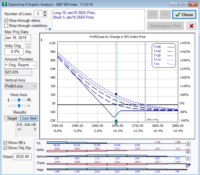
Let’s begin with an options trade, a put ratio backspread (PRBS). The OptionVue Greeks and graphical analysis as of 11/7/2018 are shown in Figures 24 and 25 below, respectively.
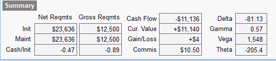
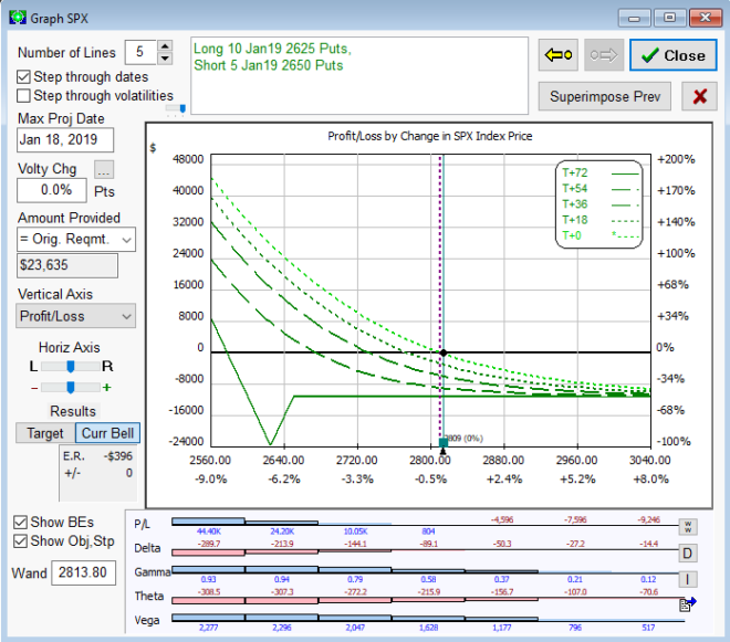
The PRBS trade required $26,636 of capital (Reg-T margin) and had the desired positive Gamma (+0.57), positive Vega (1,548), which was consistent with the volatility pricing anomalies implied by the AI Volatility Edge Analysis. You will note the Delta was also negative (-81.13). That was intentional, although adding directional exposure to volatility trades does add an additional layer of risk and requires additional conviction. Volatility and equity prices are strongly negatively correlated. Given that we are forecasting an increase in volatility, that implies the bias will be toward lower equity prices. This is why I constructed a bearish put ratio backspread example, to be consistent with our volatility forecast. However, non-directional volatility trades could definitely be used instead, one of which I will include in the alternative trade section.
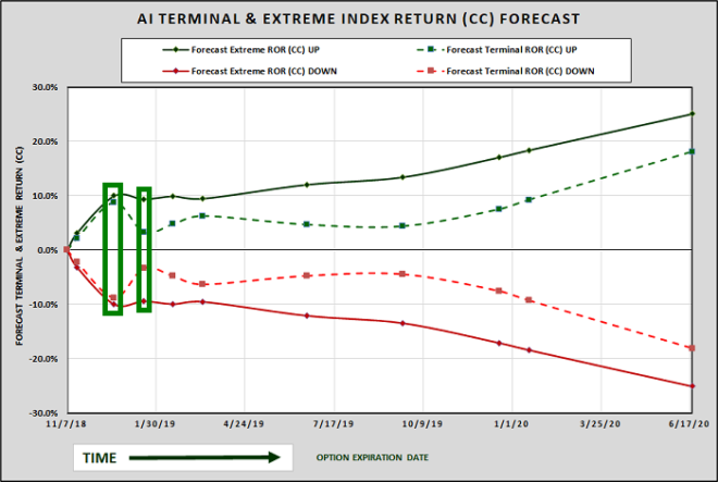
I used the Realized Terminal and Extreme Volatility price chart (Figure 26) below to estimate the potential magnitude of the price changes when selecting the strikes and designing the PRBS strategy. The AI Volatility Edge model was forecasting a 10% move in prices by December 21, far more than suggested by implied volatility at the time. The PRBS was well-positioned to profit from a large downside move in price and increase in volatility.
The narrowing of the RTV and REV forecast in January is interesting. I have noted this narrowing in a number of other near-term RTV and REV forecasts, but this occurrence was more pronounced than usual. The narrowing suggests the AIVE models have identified mean reversion in the historical price movements of the equity indices. In the case of the PRBS (a positive Gamma trade), the narrowing REV forecasts may provide an incentive to shorten our holding period.
Underpriced Volatility Trade Exit
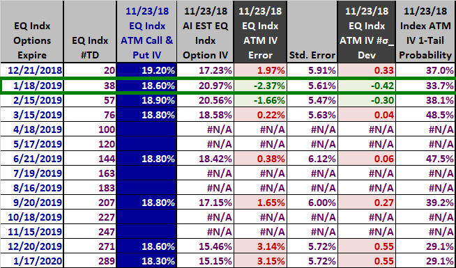
As was the case with the BWF trade, it is not practical to provide a daily analysis of the PRBS trade during the holding period, but I will provide a complete analysis on the prospective exit date for the trade: 11/23/2018. Figure 27 below compares the 11/23/2018 AI Realized Volatility forecasts to the implied volatilities for actual S&P 500 equity index options with a range of expiration dates. I have highlighted the same 1/18/2019 options expiration date that we used to construct the PRBS trade. As you can see, the ATM IV increased materially over the holding period, from 14.5% to 18.6%. While it was still slightly undervalued relative to the volatility forecasts on the proposed exit date of 11/23/2019, the z-score had increased sharply, from -1.58 to -0.42, which removed the majority of the edge from our trade.
Similarly, the degree of overvaluation had also declined to near zero (+0.01%) for the 12/19/2018 VIX futures contract (Figure 28), which further reinforced the justification for exiting the trade. The term structure of ATM implied volatilities and VIX futures prices were both overpriced in general on the exit date, although a few of the securities were still slightly underpriced.
You will recall that we used the OISUF score of negative 97.32 (and implied volatilities were below the long term mean and median) as additional support for entering the PRBS (long volatility) trade on 11/01/2018. As of 11/23/2018, the OISUF score had returned to near zero (-5.61), which would be considered a neutral volatility environment, and implied volatilities had reverted closer to the long-term mean and median values. The 11/23/2018 AI Volatility Edge forecasts and the OISUF score no longer supported an edge for the PRBS trade.
If we look at OptionVue’s graphical analysis (Figure 29) and Greeks (Figure 30) for the PRBS trade on 11/23/2018, we see that we were still well-positioned for further gains, but the magnitude of all the Greeks (Delta, Gamma, Vega, and Theta) had increased sharply since the inception of the trade, which magnified the risk. Unfortunately, the AI Volatility Edge forecasts indicated a materially smaller edge. The result: increased risk and reduced prospective return.
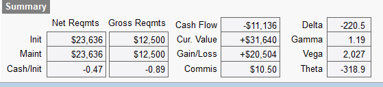
When our edge is gone – or no longer justifies the level of risk, we should exit the trade. In this case, the trade would have generated a $20,504 profit over the two-week holding period, representing a return on required capital of 86.75%.
Alternative Underpriced Volatility Trades
I will not go into the same level of detail, but I wanted to provide four alternative trades that would have been consistent with the underpriced volatility environment on 11/7/2018. The first alternative trade was a long ATM straddle using January 2019 call and put options on the SPX (anticipating a higher level of realized volatility and an increase in implied volatility). The OptionVue graphical analysis for the SPX straddle on the exit date of 11/23/2018 is shown in Figure 31 and the Greeks summary on the exit date is shown in Figure 32.
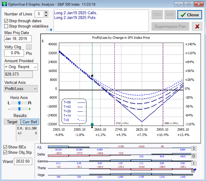
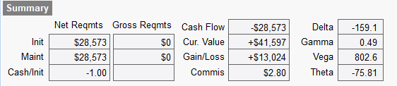
As you can see from the above exhibits, the SPX long straddle would have earned a profit of $13,024 on a capital requirement of $28,573, which would have resulted in a return on required capital of 45.58% over the two-week holding period. The long straddle would have benefited from positive Gamma and positive Vega, but was Delta-neutral at inception (unlike the PRBS trade). This explains why the PRBS trade outperformed the long straddle: the directional negative Delta at inception coupled with a large decline in the price of the SPX.
The final three alternative trades use VIX futures and VIX options, instead of SPX options to exploit the underpriced volatility environment on 11/07/2018. Note, the interpretation of the Greeks is very different for all three of these trades due to the VIX as the underlying index (instead of the S&P 500 index), which I will not explore further.
All three remaining alternative trades assume an entry on 11/07/2018 and an exit on 11/23/2018. The next alternative trade was extremely simple: the purchase of five Dec 2018 futures contracts. This is a pure long volatility strategy and has no option or SPX component. Note: unlike short volatility strategies, is not always necessary (or even desirable) to use covered strategies when being long volatility. The OptionVue graphical analysis for the long VIX futures contract on the exit date of 11/23/2018 is shown in Figure 33 and the Greeks summary on the exit date is shown in Figure 34.
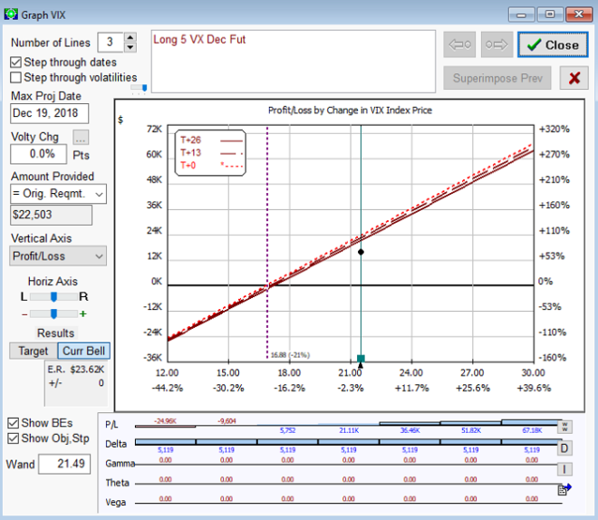
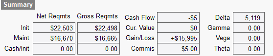
As you can see from the above exhibits, the long VIX futures strategy would have earned a profit of $15,995 on a capital requirement of $22,503 (and an initial notional value of $86,350), which would have resulted in a return on required capital of 71.08% (and a return on notional value of 18.52%) over the two-week holding period. Notional value represents value of the underlying asset or instrument in a derivatives trade. In this case, the notional value ($86,350) equals the initial price of the VIX contract ($17.27), multiplied by the size of each contract (1000), multiplied by the number of contracts traded (5).
The next alternative trade was a long Dec 2019 VIX 16 call option. The OptionVue graphical analysis for the long VIX call option on the exit date of 11/23/2018 is shown in Figure 35 and the Greeks summary on the exit date is shown in Figure 36.
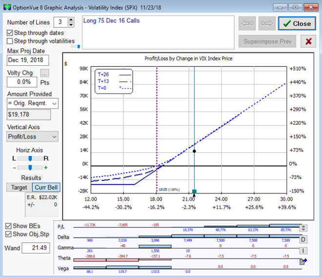
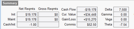
As you can see from the above exhibits, the long VIX call option would have earned a profit of $15,270 on a capital requirement of $19,178, which would have resulted in a return on required capital of 79.62% over the two-week holding period.
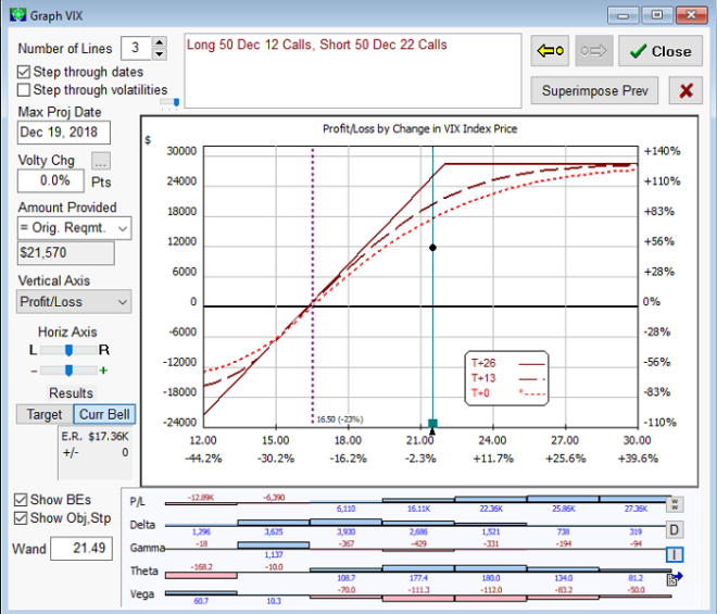
The final alternative trade was a bull call spread using Dec 2019 VIX call options. The OptionVue graphical analysis for the VIX bull call spread on the exit date of 11/23/2018 is shown in Figure 37 and the Greeks summary on the exit date is shown in Figure 38.
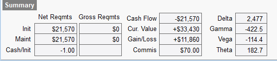
As is evident in the above exhibits, the VIX bull call spread would have earned a profit of $11,860 on a capital requirement of $21,570, which would have resulted in a return on required capital of 54.98% over the two-week holding period.
Summary
Volatility is arguably the single most important option concept, effectively determining the price of every derivatives instrument. The AI Volatility Edge platform uses the latest in machine learning algorithms to identify and quantify real-time volatility pricing anomalies that can be exploited with strategies based on SPX, NDX, and RUT index options, VIX futures, and VIX options. The AI Volatility Edge platform provides forecasts and relative value analysis across the entire term structure of volatilities.
Comprehensive AI Volatility platforms are rare, even at the institutional level. I am not aware of any other AI Volatility platforms designed by experienced investment professionals that are available on a subscription basis to professional or non-professional investors.
AI Volatility Edge (AIVE) Subscriptions
Trading Insights LLC may limit the number of AIVE subscribers at its own discretion. The proprietary AIVE volatility forecasts are run via macros in three Excel spreadsheets, which require a one-time download.
There are both non-professional and professional AIVE e-subscriptions available. The monthly subscription cost is $69 for non-professionals (individual investors) and $690 for professionals (banks, hedge funds, insurance companies, registered investment advisers, CTAs, mutual funds, endowments, pension plans, etc.). All fees are paid monthly in advance via PayPal. Subscriptions are managed via each user’s PayPal account and may be cancelled at any time. Payments are non-refundable.
The AIVE subscription is governed by a disclaimer and terms and conditions, which must be accepted prior to using the AIVE platform. The PayPal buttons below will route you to PayPal to complete the order. Once completed, you will be routed back to the Trader Edge site to complete the registration process. Please complete the registration immediately upon returning, to ensure ongoing access to the AIVE restricted/member area of the site (link).
If you have previously registered on the Trader Edge site, please use the email link you receive after ordering to register again. Please use a different email address during registration to ensure your AIVE PayPal payment profile is linked to your new registration.
Please note that a NEW version of the AIVE platform is now available and IS compatible with 64-bit versions of Excel!
The original AIVE platform is available for use with 32-bit versions of Excel (even if installed on a 64-bit version of Microsoft Windows).
Recent Changes in Availability of Free Data
When I created the OISUF and AIVE platforms, free historical daily price and IV data were available for download (export) from Yahoo and the CBOE respectively. The OISUF and AIVE platforms both have macros to import the exported Yahoo and CBOE data from exported .csv files. While the VIX data is still available for download on the CBOE site (https://www.cboe.com/tradable_products/vix/vix_historical_data/), the free historical downloads for the RVX and VXN data are not currently available on the CBOE site. Similarly, Yahoo is not currently offering free downloads for index price data. Unless and until this changes, it will not be possible to use the Yahoo and CBOE macros in the OISUF and AIVE platforms to import the historical data.
Fortunately, the AIVE platform has a separate set of macros designed to read both price and IV data from CSI, a third-party data vendor. In addition, it is always possible to copy and paste historical price and IV data from any source, directly into the OISUF and AIVE platforms.
Non-Professional: AI Volatility Edge E-Subscription: $69 / mo.
PROFESSIONAL: AI Volatility Edge E-Subscription: $690 / mo.
If you have any questions about the AIVE e-subscription or you encounter any problems during the payment or registration process, please contact Brian Johnson via email: BJohnson@TraderEdge.Net.
Brian Johnson
Brian Johnson designed, programmed, and implemented the first return sensitivity based parametric framework actively used to control risk in fixed income portfolios. He further extended the capabilities of this approach by designing and programming an integrated series of option valuation, prepayment, and portfolio optimization models.
Based on this technology, Mr. Johnson founded Lincoln Capital Management’s fixed income index business, where he ultimately managed over $13 billion in assets for some of the largest and most sophisticated institutional clients in the U.S. and around the globe.
He later served as the President of a financial consulting and software development firm, designing artificial intelligence-based forecasting and risk management systems for institutional investment managers.
Mr. Johnson is now a full-time proprietary trader in options, futures, stocks, and ETFs primarily using algorithmic trading strategies. In addition to his professional investment experience, he also designed and taught courses in financial derivatives for MBA, Masters of Accounting, and undergraduate business programs - most recently as a Professor of Practice at the University of North Carolina’s Kenan-Flagler Business School.
He is the author of two groundbreaking books on options: 1) Option Strategy Risk / Return Ratios: A Revolutionary New Approach to Optimizing, Adjusting, and Trading Any Option Income Strategy, and 2) Exploiting Earnings Volatility: An Innovative New Approach to Evaluating, Optimizing, and Trading Option Strategies to Profit from Earnings Announcements.
He recently authored two in-depth (100+ page) articles on option strategy. The first, Option Income Strategy Trade Filters, represents the culmination of years of research into developing a systematic framework for optimizing the timing of Option Income Strategy (OIS) trades. The second, Option Strategy Hedging and Risk Management, presents a comprehensive analytical framework and accompanying spreadsheet tools for managing and hedging option strategy risk in real-world market environments.
He has also written articles for the Financial Analysts Journal, Active Trader, and Seeking Alpha and he regularly shares his trading insights and research ideas as the editor of https://www.traderedge.net/.
Mr. Johnson holds a B.S. degree in Finance with high honors from the University of Illinois at Urbana-Champaign and an MBA degree with a specialization in Finance from the University of Chicago Booth School of Business.
Email: BJohnson@TraderEdge.Net