As traders, there are very few things we know with certainty. But there are several factors that we can forecast accurately - even years in advance:
- when domestic and international holidays will occur
- when economic data will be released
- when earnings season will occur
- when income taxes will be due
- when monthly and semi-monthly paychecks will be issued
- when temperatures will be relatively high or relatively low
- when crops will be planted and when they will be harvested
- etc.
All of the above events (and many others) occur at regular seasonal intervals and they all affect the natural supply and demand cycles in the financial and commodity markets. How can we harness the power of these seasonal tendencies to improve our investment performance?
CAR Seasonal Indicator
Before we can integrate seasonality into our investment process, we need to create an objective tool to measure the historical, seasonal price performance for each market. In many cases, seasonality is depicted by a single normalized line on a graph.
To determine the seasonal trend with these types of graphs, we must visually compare the current level to some future point on the graph. Unfortunately, the scales are often poorly defined and difficult to translate into risk and return. This makes it challenging to identify the strongest and weakest seasonal candidates among a group of individual securities or futures contracts.
To address these deficiencies, I created two different seasonal indicators. The first calculates the average compound annual return (CAR) for a user-specified holding period over the historical time period chosen by the user.
For example, let's assume that we wanted to evaluate 4-week holding periods since 1990. The indicator would calculate the average compound annual return for each week of the year for the period 1990 to present. In other words, there would be 52 separate CAR values, one for each week of the year. The resulting CAR values would be directly comparable across securities and over different investment horizons, which would allow us to use this indicator to create specific objective decision rules.
While compound annual return is easy to understand, it is affected by volatility. More volatile securities will have wider seasonal CAR ranges than less volatile securities. That is the reason that I calculated a second seasonal indicator: a modified version of the "profit factor."
Modified Profit Factor (MPF)
Profit factor is a common metric used to evaluate the success of a strategy over a specified time period. Profit factor equals the cumulative gains for the strategy divided by the absolute value of cumulative losses (cumulative gains / ABS(cumulative losses)).
If cumulative gains were exactly offset by cumulative losses, the resulting profit factor would be 1.0. A profit factor of 4.0 would signify that cumulative gains were four times the magnitude of cumulative losses. Conversely, a profit factor of 0.25 would indicate that cumulative losses were four times the magnitude of cumulative gains. As you can see, the industry standard profit factor calculation is centered at 1.0, but is not symmetric around 1.0.
I wanted a seasonal indicator that was symmetric, so I could use comparable decision rules to evaluate long and short positions. That is the reason that I created the modified profit factor (MFP), which is centered at 0.0 and is also symmetric.
If cumulative gains > cumulative losses:
- MPF = (cumulative gains / ABS(cumulative losses)) - 1.0
If cumulative gains <= cumulative losses:
- MPF = (-ABS(cumulative losses) / cumulative gains) + 1.0
A MPF of 3.0 would mean that cumulative losses are 300% higher or four times the magnitude of cumulative losses. In this example, if cumulative losses were - 20%, cumulative gains would equal 80%. A MPF of -3.0 would correspond to cumulative gains of 20% and cumulative losses of -80%. As you can see, the MPF is symmetric around 0.0.
To calculate the MPF seasonal indicator, the user must again specify the holding period and the historical time period to calculate the returns. However, instead of using the return data to calculate the average compound annual return, the same return data are used to calculate the MPF, using the formula above.
Sell in May and Go Away
We have all heard the maxim, "sell in May and go away." The saying implies that the seasonal returns for the equity market are negative during the summer months and turn positive again in the fall and stay positive until the following May. Is this well-known guideline supported by the historical data?
To find out, I calculated the CAR and MPF seasonal indicators for the e-mini S&P futures contract using a 4-week holding period. I calculated these values over a custom historical period, which I will explain in more detail at the end of the article.
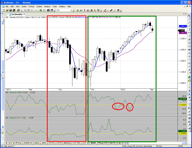
The top panel in Figure 1 below is a weekly candlestick chart of price of the e-mini S&P futures contract. The second panel is a graph of the seasonal CAR for each week of the year; the CAR scale can be found on the right-hand-side axis. The yellow horizontal line is the zero line. Values above the zero line represent positive CARs and values below the zero line represent negative CARs.
The bottom panel is a graph of the MPF for each week of the year. The MPF scale is on the axis to the right. Again, the yellow horizontal line is the zero MPF line.
Except for one brief week in the period from 5/27 through 9/23 (inside the red box below), the historical CAR and MPF values were all negative. The historical performance for some of the weeks in this period was terrible, with CAR values below -20% and MPF values below -1.5.
Conversely, the CAR and MPF values were predominately positive in the period from 9/30 through 5/20 (inside the green box below). There were a few weeks in late December and early February when the CAR and MPF dipped below zero, but they were exceptions to the rule. The vast majority of weeks were positive. In several cases, the CAR values exceeded 20%. A few of the MPF values were extremely high; one week had an MPF value over 6.0. This means that cumulative gains for this week historically were seven times the magnitude of cumulative losses - a remarkable advantage for bullish positions.
Were the results for the e-mini S&P 500 contract in 2011 consistent with the historical CAR and MPF seasonal indicators? I did not conduct a statistical analysis, but the overall results are apparent from looking at the chart. The market did indeed perform poorly from late May through September of 2011 and performed extremely well from late September 2011 through the second week of April 2012.
Seasonal Patterns in the Gold Market
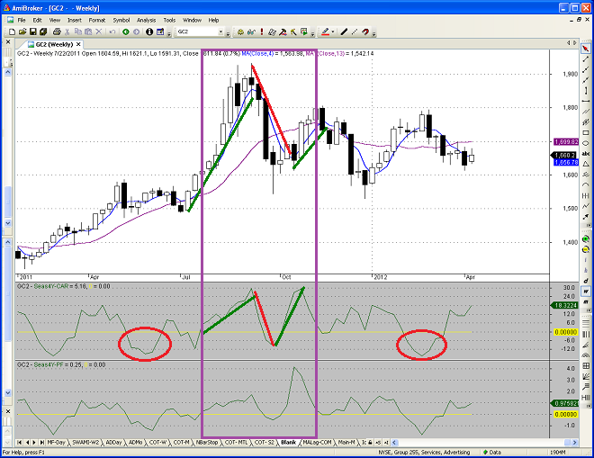
Figure 2 below is a weekly chart of the continuous gold futures contract from early 2011 through the second week of April 2012. The format is the same as in Figure 1: candlestick chart, CAR indicator, and MPF indicator (top to bottom).
As you can see below, "sell in May and go way" does not apply to the gold market. This is an important observation: every market has its own unique seasonal pattern driven by natural supply and demand relationships.
Given the extended bull market in gold, it is not surprising to find very few negative CAR and MPF seasonal periods below. However, two of these weak seasonal periods are circled in red below. Historically, gold prices have tended to decline from mid-February to mid-March and throughout the month of May.
Occasionally, prices will track the seasonal indicator values very closely. In the purple box above, notice how closely the price of gold followed the seasonal CAR and MPF indicators from July through October 2011.
Practical Considerations
The CAR and MPF values in charts above were based on 4-week holding periods. However, I did not use a single historical time period to calculate the returns. I went back to the 1980s, but I assigned more weight to recent historical data, recognizing the fact that seasonal patterns may evolve over time. That is the advantage of creating our own indicators - the ability to customize tools to meet our specific needs.
You could use the CAR and MPF indicators to create objective decision or filter rules. For example, never enter a long position when the MPF is less than 0.0, or less than -1.0, or less than +1.0. The choice is up to you. You could even use multiple filters, each with a different investment horizon.
More restrictive filters would reduce your number of trades, but should increase your percentage of winning trades. The CAR and MPF seasonal indicators were designed with user-defined parameters that could be used to back-test mechanical trading strategies. Experiment with different parameters and find the best fit for your investment process.
The golden rule of trading is to always trade with the existing trend. You could use seasonal indicators to always trade with the seasonal trend as well. If you want to further improve your probability of success, consider adding overbought or oversold filters to your trading strategy.
The CAR and MPF values are directly comparable across different markets. As a result, you could scan groups of securities or futures contracts to identify the best bullish or bearish seasonal prospects. Remember that each market has a different seasonal pattern. Individual stocks and sector ETFs may have very different seasonal patterns than the broad market indices. Unfortunately, most ETFs have a very limited history, while there are many years of data available for futures contracts and many individual stocks.
While seasonal indicators are powerful tools, I would not base investment decisions exclusively on past seasonal price patterns. However, when used in conjunction with other technical and fundamental tools, they could dramatically improve your investment results and reduce your losses
Feedback
Your comments, feedback, and questions are always welcome and appreciated. Please use the comment section at the bottom of this page or send me an email.
Do you have any questions about the material? What topics would you like to see in the future?
Referrals
If you found the information on www.TraderEdge.Net helpful, please pass along the link to your friends and colleagues or share the link with your social network.
The "Share / Save" button below contains links to all major social networks. If you do not see your social network listed, use the down-arrow to access the entire list of social networking sites.
Thank you for your support.
Brian Johnson
Copyright 2012 - Trading Insights, LLC - All Rights Reserved.
.


Pingback: Happy Hour: Booze Will Save The Post Office & $50K To Happiness • Novel Investor
Pingback: Are the Seasonal Trends Working this Year? | Trader Edge