I read an interesting article by Neil Azous in the December 2015 issue of Modern Trader ("Has the Golden Moment Passed?") that inspired me to do some further research into modeling gold prices. The resulting research greatly enhanced my understanding of the fundamental drivers of gold prices and even corrected several misconceptions that I have carried with me for the past 30 years.
Explaining Gold Prices
The author of the article (Azous) ran two regressions. The first regression used seven explanatory variables to explain gold prices. The second regression used changes in the same seven variables to model changes in the price of gold. The author's independent or explanatory variables included:
- Real 10-year yield
- U.S Dollar (DXY)
- Volatility (VIX)
- Central Bank Gold buys
- Industrial metals price
- Annual CPI - 1.5%
- ISM Manufacturing - 50
I analyzed the author's regression results and made several changes to the regression models. First, I excluded variables that had inconsistent signs in the two regressions. For example, the regression coefficient for central bank gold buys was positive in the first regression and negative in the second regression, which is contradictory. I excluded all such variables. I also excluded variables from both regressions that were not statistically significant (marginal T-statistic) in one or both of the regressions.
In addition, I also eliminated variables that were not practical. For example, there is no question that the price of gold is correlated with the price of industrial metals. However, when using the regression results as a forecasting tool, I would be required to enter the assumed future price for industrial metals. It seemed unreasonable for me to enter the future price for industrial metals to forecast the future price of gold.
Finally, I combined the real 10-year yield with the annual CPI variables into a single explanatory variable: the nominal yield of the 10-year UST note. Before doing so, I confirmed that the regression coefficients for both variables were almost identical and had comparable explanatory power. Whenever possible, it is preferable to limit the number of independent regression variables.
The resulting regressions only had two underlying explanatory variables: the nominal 10-year UST yield and the U.S. Dollar index. I used natural log transformations on all variables to improve the fit of the regression models and to eliminate the potential for negative gold prices in the model.
The regression results were statistically significant and very instructive.
Gold Price Regression
As a reminder, the first regression used the nominal yield of the 10-year UST note and the U.S. Dollar index to explain the spot price of gold. The regression period included monthly data from December 1985 to December 2015, 30 years of monthly data. The R squared value for the regression was 0.7874, which indicates that 78.74% of the variation in the price of gold was explained by the regression - a very powerful result for only two explanatory variables.
The absolute value of the t-statistics for the intercept and two beta coefficients were all above 15. The beta coefficients for the Nominal 10-year UST yield and the U.S. Dollar Index were both negative and highly significant. In other words, there is no question that there is an inverse relationship between the 10-year UST yields and the price of gold and between the U.S. Dollar index and the price of gold.
As 10-year yields increase (due to changes in inflation or real yields), the price of gold falls. Similarly, increases in the value of the U.S. Dollar correspond to declines in the price of gold.
Change in Gold Price Regression
The second regression used changes in the nominal yield of the 10-year UST note and changes in the U.S. Dollar index to explain percentage changes in the spot price of gold. The regression period included 35-month data periods from October 1988 to December 2015, 30 years of monthly data.
Why did I use 35-month periods? Because technical factors dominate fundamental factors in the short-term. The importance of fundamental factors increases with time, as the relative importance of the short-term noise diminishes. Using intermediate-term periods makes it much easier to quantify the impact of the explanatory variables on gold returns.
The R squared value for the regression was 0.4333, which indicates that 43.31% of the variation in the percentage change in the price of gold was explained by the regression. This was not as powerful as the first regression, but still impressive for a two variable model.
The absolute value of the t-statistics for the two beta coefficients were all above 9.5. The beta coefficients for the changes in the nominal 10-year UST yield and changes in the U.S. Dollar Index were both negative and highly significant. As was the case in the first regression, there is no question that there is an inverse relationship between the 10-year UST yields and the price of gold and between the U.S. Dollar index and the price of gold.
Gold is Still Overvalued
Now that I have explained the regression model framework, let's look at the results. The blue line in Figure 1 below represents the monthly regression model estimates for the spot price of gold from December 1, 1985 to December 1, 2015. The purple line in Figure 1 below represents the spot price of gold over the same period. When the blue (model price) line is above the purple (spot price) line, gold is undervalued or cheap. When the blue (model price) line is below the purple (spot price) line, gold is overvalued or rich.

Figure 1: Gold Prices 12-1-2015
I also included a second chart below in Figure 2 to make it easier to see the magnitude of overvaluation or undervaluation. Positive values indicate that gold is undervalued (Model > Spot) and negative values represent periods when gold was overvalued (Model < Spot). These values are expressed in percentage terms, which represent the return to gold if the spot price instantaneously corrected to the model price.
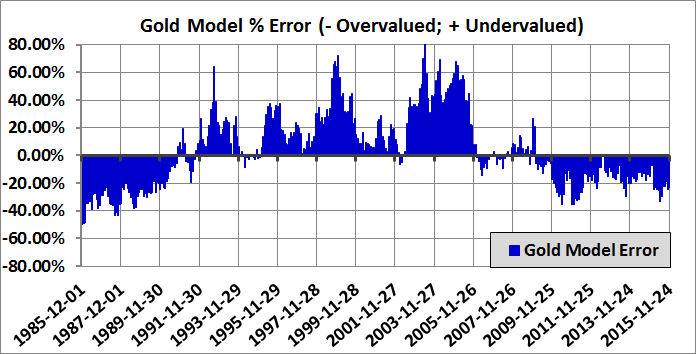
Figure 2: Gold Regression Model Errors 12-1-2015
Conclusion
I already knew that gold prices were inversely related to the price of the U.S. Dollar. However, I am embarrassed to admit that I still believed that gold prices were positively influenced by inflation. In other words, I believed the standard gold bug sales pitch: gold is an inflation hedge. It certainly sounded plausible and I knew/remembered that the high levels of inflation in the late 70s and early 80s were associated with a very large spike in the price of gold. While my recollection was accurate, the positive relationship between inflation and gold prices has not held for over 30 years.
Increases in both real yield AND inflation have resulted in decreases in gold prices for the past 30 years. One caveat: the maximum nominal 10-year UST yield in the above data set was only 9.5%. It would be dangerous to extrapolate this regression model for yields above 9.5%.
The regression model also provides objective, real-time information on the value of gold. As of December 1, 2015, the regression model indicates that gold is still overvalued by 23.55%, even after suffering a 42% decline over the past five years - not good news for the gold bugs. If the dollar continues to increase in value and 10-year UST rates continue to rise, the implications for gold would be even worse.
Print and Kindle Versions of Brian Johnson's 2nd Book are Available on Amazon (75% 5-Star Reviews)
Exploiting Earnings Volatility: An Innovative New Approach to Evaluating, Optimizing, and Trading Option Strategies to Profit from Earnings Announcements.
Print and Kindle Versions of Brian Johnson's 1st Book are Available on Amazon (79% 5-Star Reviews)
Option Strategy Risk / Return Ratios: A Revolutionary New Approach to Optimizing, Adjusting, and Trading Any Option Income Strategy
Trader Edge Strategy E-Subscription Now Available: 20% ROR
The Trader Edge Asset Allocation Rotational (AAR) Strategy is a conservative, long-only, asset allocation strategy that rotates monthly among five large asset classes. The AAR strategy has generated annual returns of approximately 20% over the combined back and forward test period. Please use the above link to learn more about the AAR strategy.
Brian Johnson
Copyright 2015 - Trading Insights, LLC - All Rights Reserved.


Gold Still Overvalued by 23.5%
I read an interesting article by Neil Azous in the December 2015 issue of Modern Trader ("Has the Golden Moment Passed?") that inspired me to do some further research into modeling gold prices. The resulting research greatly enhanced my understanding of the fundamental drivers of gold prices and even corrected several misconceptions that I have carried with me for the past 30 years.
Explaining Gold Prices
The author of the article (Azous) ran two regressions. The first regression used seven explanatory variables to explain gold prices. The second regression used changes in the same seven variables to model changes in the price of gold. The author's independent or explanatory variables included:
I analyzed the author's regression results and made several changes to the regression models. First, I excluded variables that had inconsistent signs in the two regressions. For example, the regression coefficient for central bank gold buys was positive in the first regression and negative in the second regression, which is contradictory. I excluded all such variables. I also excluded variables from both regressions that were not statistically significant (marginal T-statistic) in one or both of the regressions.
In addition, I also eliminated variables that were not practical. For example, there is no question that the price of gold is correlated with the price of industrial metals. However, when using the regression results as a forecasting tool, I would be required to enter the assumed future price for industrial metals. It seemed unreasonable for me to enter the future price for industrial metals to forecast the future price of gold.
Finally, I combined the real 10-year yield with the annual CPI variables into a single explanatory variable: the nominal yield of the 10-year UST note. Before doing so, I confirmed that the regression coefficients for both variables were almost identical and had comparable explanatory power. Whenever possible, it is preferable to limit the number of independent regression variables.
The resulting regressions only had two underlying explanatory variables: the nominal 10-year UST yield and the U.S. Dollar index. I used natural log transformations on all variables to improve the fit of the regression models and to eliminate the potential for negative gold prices in the model.
The regression results were statistically significant and very instructive.
Gold Price Regression
As a reminder, the first regression used the nominal yield of the 10-year UST note and the U.S. Dollar index to explain the spot price of gold. The regression period included monthly data from December 1985 to December 2015, 30 years of monthly data. The R squared value for the regression was 0.7874, which indicates that 78.74% of the variation in the price of gold was explained by the regression - a very powerful result for only two explanatory variables.
The absolute value of the t-statistics for the intercept and two beta coefficients were all above 15. The beta coefficients for the Nominal 10-year UST yield and the U.S. Dollar Index were both negative and highly significant. In other words, there is no question that there is an inverse relationship between the 10-year UST yields and the price of gold and between the U.S. Dollar index and the price of gold.
As 10-year yields increase (due to changes in inflation or real yields), the price of gold falls. Similarly, increases in the value of the U.S. Dollar correspond to declines in the price of gold.
Change in Gold Price Regression
The second regression used changes in the nominal yield of the 10-year UST note and changes in the U.S. Dollar index to explain percentage changes in the spot price of gold. The regression period included 35-month data periods from October 1988 to December 2015, 30 years of monthly data.
Why did I use 35-month periods? Because technical factors dominate fundamental factors in the short-term. The importance of fundamental factors increases with time, as the relative importance of the short-term noise diminishes. Using intermediate-term periods makes it much easier to quantify the impact of the explanatory variables on gold returns.
The R squared value for the regression was 0.4333, which indicates that 43.31% of the variation in the percentage change in the price of gold was explained by the regression. This was not as powerful as the first regression, but still impressive for a two variable model.
The absolute value of the t-statistics for the two beta coefficients were all above 9.5. The beta coefficients for the changes in the nominal 10-year UST yield and changes in the U.S. Dollar Index were both negative and highly significant. As was the case in the first regression, there is no question that there is an inverse relationship between the 10-year UST yields and the price of gold and between the U.S. Dollar index and the price of gold.
Gold is Still Overvalued
Now that I have explained the regression model framework, let's look at the results. The blue line in Figure 1 below represents the monthly regression model estimates for the spot price of gold from December 1, 1985 to December 1, 2015. The purple line in Figure 1 below represents the spot price of gold over the same period. When the blue (model price) line is above the purple (spot price) line, gold is undervalued or cheap. When the blue (model price) line is below the purple (spot price) line, gold is overvalued or rich.
Figure 1: Gold Prices 12-1-2015
I also included a second chart below in Figure 2 to make it easier to see the magnitude of overvaluation or undervaluation. Positive values indicate that gold is undervalued (Model > Spot) and negative values represent periods when gold was overvalued (Model < Spot). These values are expressed in percentage terms, which represent the return to gold if the spot price instantaneously corrected to the model price.
Figure 2: Gold Regression Model Errors 12-1-2015
Conclusion
I already knew that gold prices were inversely related to the price of the U.S. Dollar. However, I am embarrassed to admit that I still believed that gold prices were positively influenced by inflation. In other words, I believed the standard gold bug sales pitch: gold is an inflation hedge. It certainly sounded plausible and I knew/remembered that the high levels of inflation in the late 70s and early 80s were associated with a very large spike in the price of gold. While my recollection was accurate, the positive relationship between inflation and gold prices has not held for over 30 years.
Increases in both real yield AND inflation have resulted in decreases in gold prices for the past 30 years. One caveat: the maximum nominal 10-year UST yield in the above data set was only 9.5%. It would be dangerous to extrapolate this regression model for yields above 9.5%.
The regression model also provides objective, real-time information on the value of gold. As of December 1, 2015, the regression model indicates that gold is still overvalued by 23.55%, even after suffering a 42% decline over the past five years - not good news for the gold bugs. If the dollar continues to increase in value and 10-year UST rates continue to rise, the implications for gold would be even worse.
Print and Kindle Versions of Brian Johnson's 2nd Book are Available on Amazon (75% 5-Star Reviews)
Exploiting Earnings Volatility: An Innovative New Approach to Evaluating, Optimizing, and Trading Option Strategies to Profit from Earnings Announcements.
Print and Kindle Versions of Brian Johnson's 1st Book are Available on Amazon (79% 5-Star Reviews)
Option Strategy Risk / Return Ratios: A Revolutionary New Approach to Optimizing, Adjusting, and Trading Any Option Income Strategy
Trader Edge Strategy E-Subscription Now Available: 20% ROR
The Trader Edge Asset Allocation Rotational (AAR) Strategy is a conservative, long-only, asset allocation strategy that rotates monthly among five large asset classes. The AAR strategy has generated annual returns of approximately 20% over the combined back and forward test period. Please use the above link to learn more about the AAR strategy.
Brian Johnson
Copyright 2015 - Trading Insights, LLC - All Rights Reserved.
About Brian Johnson
I have been an investment professional for over 30 years. I worked as a fixed income portfolio manager, personally managing over $13 billion in assets for institutional clients. I was also the President of a financial consulting and software development firm, developing artificial intelligence based forecasting and risk management systems for institutional investment managers. I am now a full-time proprietary trader in options, futures, stocks, and ETFs using both algorithmic and discretionary trading strategies. In addition to my professional investment experience, I designed and taught courses in financial derivatives for both MBA and undergraduate business programs on a part-time basis for a number of years. I have also written four books on options and derivative strategies.